Resonance Measurement

The analysis module provides tools for performing resonance measurements using the NV200 device. It includes the ResonanceAnalyzer class, which simplifies the process of measuring and analyzing the device’s impulse response.

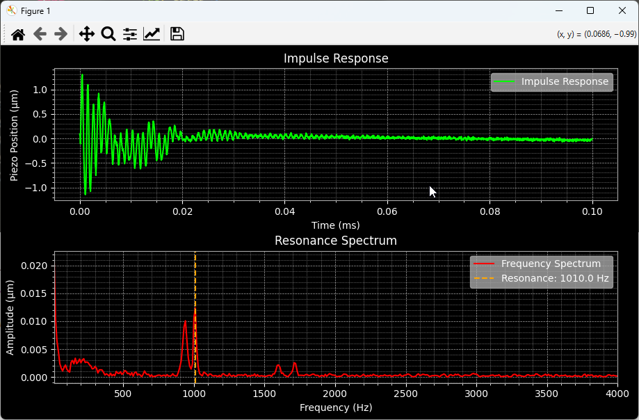
The following example demonstrates how to use the nv200.analysis module with the NV200Device. It covers connecting to the device, measuring the impulse response, computing the resonance spectrum, and visualizing the results using matplotlib.

from nv200.nv200_device import NV200Device
from nv200.shared_types import TransportType
from nv200.analysis import ResonanceAnalyzer
from nv200.connection_utils import connect_to_single_device

import matplotlib_helpers

async def resonance_measurement_test():
    # Connect to the one and only NV200 device connected via serial port
    dev = await connect_to_single_device(NV200Device, TransportType.SERIAL)

    # Create resonance analyzer for the connected device
    analyzer = ResonanceAnalyzer(dev)

    # first measure impulse response and then use it to compute the resonance spectrum
    signal, sample_freq, rec_src = await analyzer.measure_impulse_response()
    xf, yf, res_freq = ResonanceAnalyzer.compute_resonance_spectrum(signal, sample_freq)

    # Get the position unit from the device for showing the unit in the plot
    unit = await dev.get_position_unit()

    # Use matplotlib to plot the recorded data
    t = np.arange(len(signal)) / sample_freq  # time in seconds

    # Create figure with 2 subplots (rows=2, cols=1)
    plt.style.use('dark_background')
    fig, (ax1, ax2) = plt.subplots(2, 1, figsize=(10, 6), sharex=False)

    # Plot impulse response into first subplot
    ax1.plot(t, signal, color=(0.0, 1.0, 0.0), label='Impulse Response')
    ax1.set_xlabel("Time (ms)")
    ax1.set_ylabel(f"Piezo Position ({unit})")
    ax1.set_title("Impulse Response")
    matplotlib_helpers.prepare_axes_style(ax1)

    # Plot frequency spectrum into second subplot
    ax2.plot(xf, yf, color='r', label='Frequency Spectrum')
    ax2.axvline(float(res_freq), color='orange', linestyle='--', label=f'Resonance: {float(res_freq):.1f} Hz')
    ax2.set_xlabel("Frequency (Hz)")
    ax2.set_ylabel(f"Amplitude ({unit})")
    ax2.set_title("Resonance Spectrum")
    ax2.set_xlim(10, 4000)
    matplotlib_helpers.prepare_axes_style(ax2)

    plt.tight_layout()
    plt.show(block=True)

Step by Step Guide to Performing a Resonance Measurement

This guide will walk you through the steps to connect to an NV200 device, measure its impulse response, compute the resonance spectrum, and visualize the results.

Step 1: Import Necessary Modules

Start by importing all required modules. This includes the NV200 device classes, analysis tools, connection utilities, and any plotting helpers.

import asyncio
import numpy as np
import matplotlib.pyplot as plt

from nv200.nv200_device import NV200Device
from nv200.shared_types import TransportType
from nv200.analysis import ResonanceAnalyzer
from nv200.connection_utils import connect_to_single_device
import matplotlib_helpers

Step 2: Connect to the NV200 Device

Establish a connection to a single NV200 device. In this example, we use a serial transport.

dev = await connect_to_single_device(NV200Device, TransportType.SERIAL)
print(f"Connected to device: {dev.name}")

Step 3: Create the Resonance Analyzer

Create an instance of ResonanceAnalyzer using the connected device. This will handle measurement of the impulse response and computation of the resonance spectrum.

analyzer = ResonanceAnalyzer(dev)

Step 4: Measure Impulse Response

Measure the device’s impulse response using the analyzer. This function returns the signal, sampling frequency, and the recording source.

signal, sample_freq, rec_src = await analyzer.measure_impulse_response()

Attention

The impulse response measurement will create a short impulse from a Base Voltage to a Peak Voltage to get the impulse response from the device. Ensure that the resulting motion or force cannot damage your application or surrounding equipment.

Step 5: Compute the Resonance Spectrum

Compute the resonance spectrum from the measured impulse response. This returns the frequency array, amplitude spectrum, and the resonance frequency.

xf, yf, res_freq = ResonanceAnalyzer.compute_resonance_spectrum(signal, sample_freq)

Step 6: Retrieve Device Units

Get the position unit from the device to label your plots accurately.

unit = await dev.get_position_unit()

Step 7: Prepare Data for Plotting

Calculate the time axis for the impulse response. Set up the figure and subplots.

t = np.arange(len(signal)) / sample_freq  # time in seconds
plt.style.use('dark_background')
fig, (ax1, ax2) = plt.subplots(2, 1, figsize=(10, 6), sharex=False)

Step 8: Plot Impulse Response

Plot the measured impulse response in the first subplot.

ax1.plot(t, signal, color=(0.0, 1.0, 0.0), label='Impulse Response')
ax1.set_xlabel("Time (ms)")
ax1.set_ylabel(f"Piezo Position ({unit})")
ax1.set_title("Impulse Response")
matplotlib_helpers.prepare_axes_style(ax1)

Step 9: Plot Resonance Spectrum

Plot the computed resonance spectrum in the second subplot, including a line for the detected resonance frequency.

ax2.plot(xf, yf, color='r', label='Frequency Spectrum')
ax2.axvline(float(res_freq), color='orange', linestyle='--', label=f'Resonance: {float(res_freq):.1f} Hz')
ax2.set_xlabel("Frequency (Hz)")
ax2.set_ylabel(f"Amplitude ({unit})")
ax2.set_title("Resonance Spectrum")
ax2.set_xlim(10, 4000)
matplotlib_helpers.prepare_axes_style(ax2)

Step 10: Display the Plots

Finalize the layout and show the plots. The block=True argument ensures the figure stays open.

plt.tight_layout()
plt.show(block=True)

API Reference

You will find a detailed description of the API methods and their usage in the API Reference.